
CuDAFLOW: CUDA Discrete-Adjoint CFD

🔍 Project Overview
CuDAFLOW is a single-precision GPU finite-volume compressible RANS/LES solver built around an exact discrete adjoint. Its distinguishing piece is CuAD, a Tapenade-style source-to-source automatic-differentiation compiler for CUDA (Clang LibTooling): CuAD differentiates the actual GPU residual kernels, so every derivative in the adjoint chain is exact rather than finite difference.
- Flow solver (GPU, FP32) — structured multiblock, overset/chimera, AUSMPW+ with up to 5th-order MUSCL / eMLP-VC reconstruction, full viscous fluxes, Spalart–Allmaras (RANS) and SA-DDES/IDDES/Vreman (LES), implicit red-black / line (DADI) smoothing and pseudo-time multigrid, dual-time unsteady.
- CuAD — CUDA AD compiler (now a separate open-source repository) — forward (tangent) and reverse (adjoint) mode; handles arrays, structs, cross-call,
atomicAdd, ternaries and 2-D array access. It differentiates the heavy flux/viscous/turbulence kernels exactly. - Exact discrete adjoint — the stiff RANS adjoint amplifies any finite-difference term by the condition number, so all four amplified derivatives — the Jacobian ∂R/∂Q, the objective seed ∂J/∂Q, the mesh sensitivity ∂R/∂X and the wall-distance term ∂R/∂wd — are produced by CuAD AD. A 6.85%-accurate FP32 finite-difference Jacobian gave a shape gradient 233× too large and the wrong sign; the full-AD chain recovers the correct sign and magnitude.
- Optimization from Python — objectives
cd, cl, cf, cp, qwand design variables (FFD control points or the SA field β), driven by pyOptSparse. Objective and constraints are plain Python callables of the CFD functionals. - PETSc adjoint solve — the assembled block Jacobian is solved in double precision with GMRES + ILU (the only FP64 part; the flow stays FP32).
✅ Validation Status
| Case | Configuration | Result |
|---|---|---|
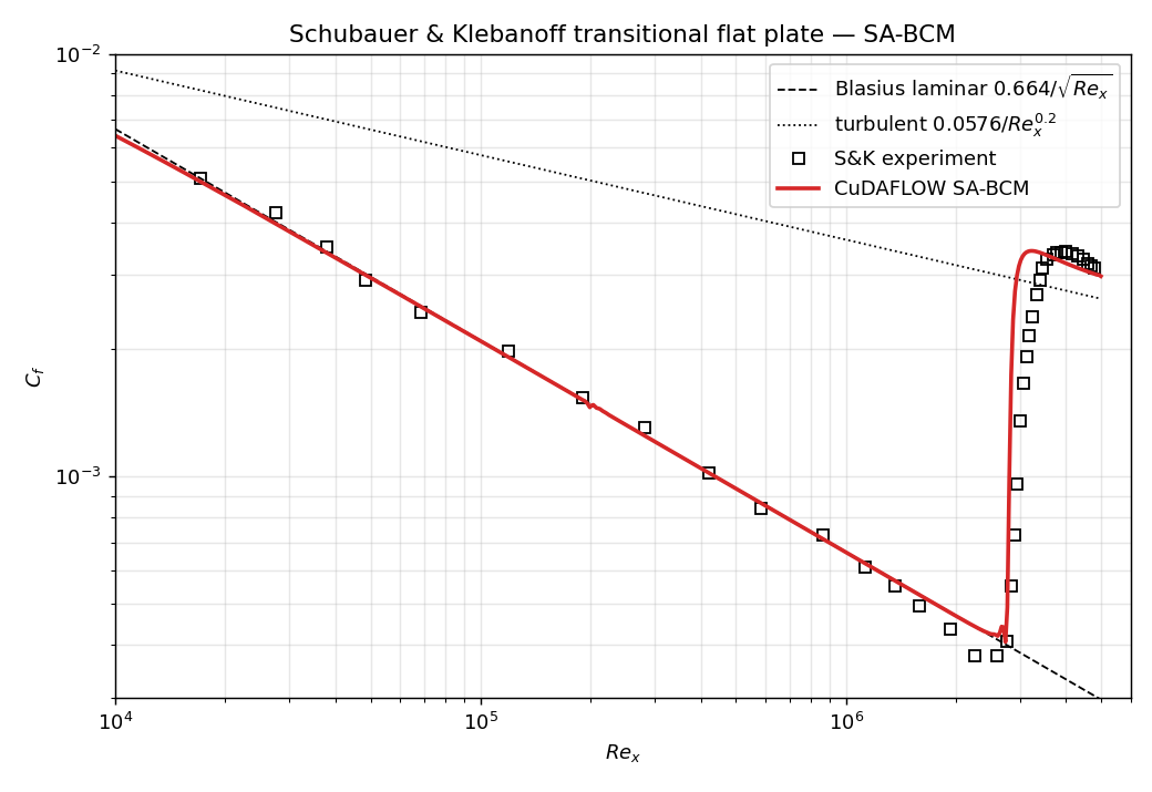
| Schubauer–Klebanoff flat plate | SA-BCM transition, M = 0.3, LE-refined grid | Skin friction matches the S&K transitional experiment |
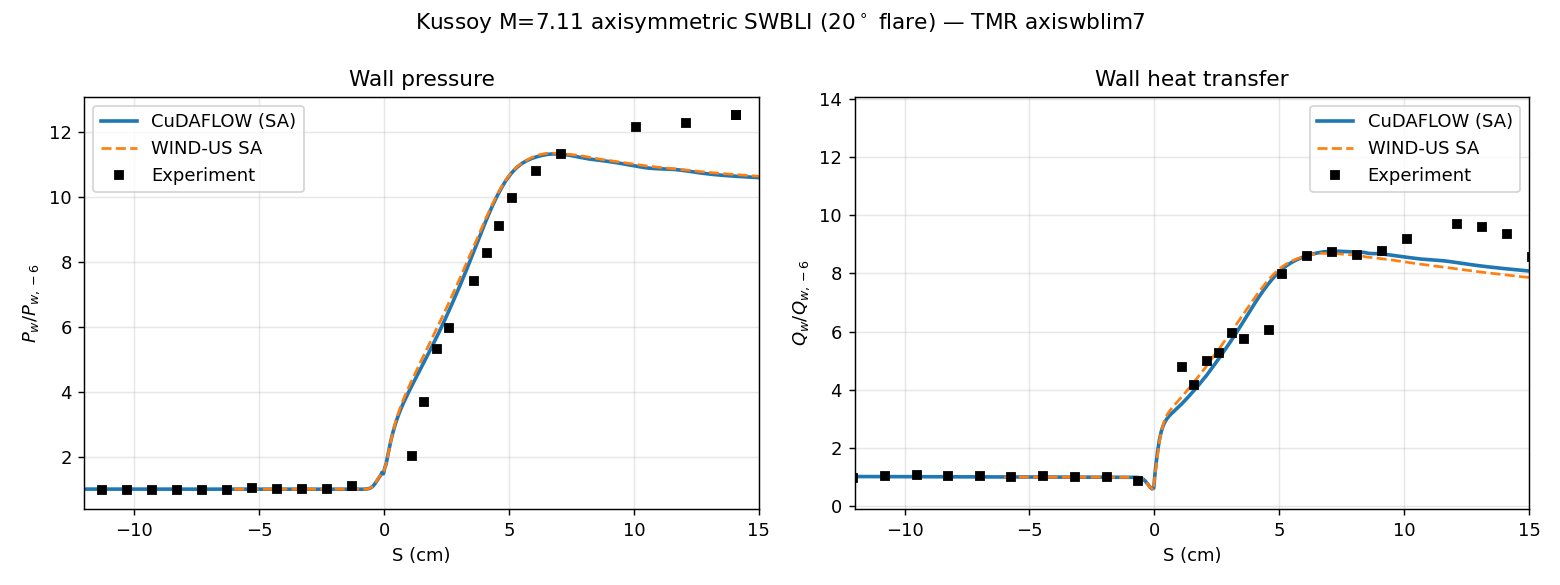
| Axisymmetric Mach-7 SWBLI (Kussoy) | Spalart–Allmaras, Re = 57 000 / cm | Wall pressure / heating within ~1–2% of the reference WIND-SA solution |
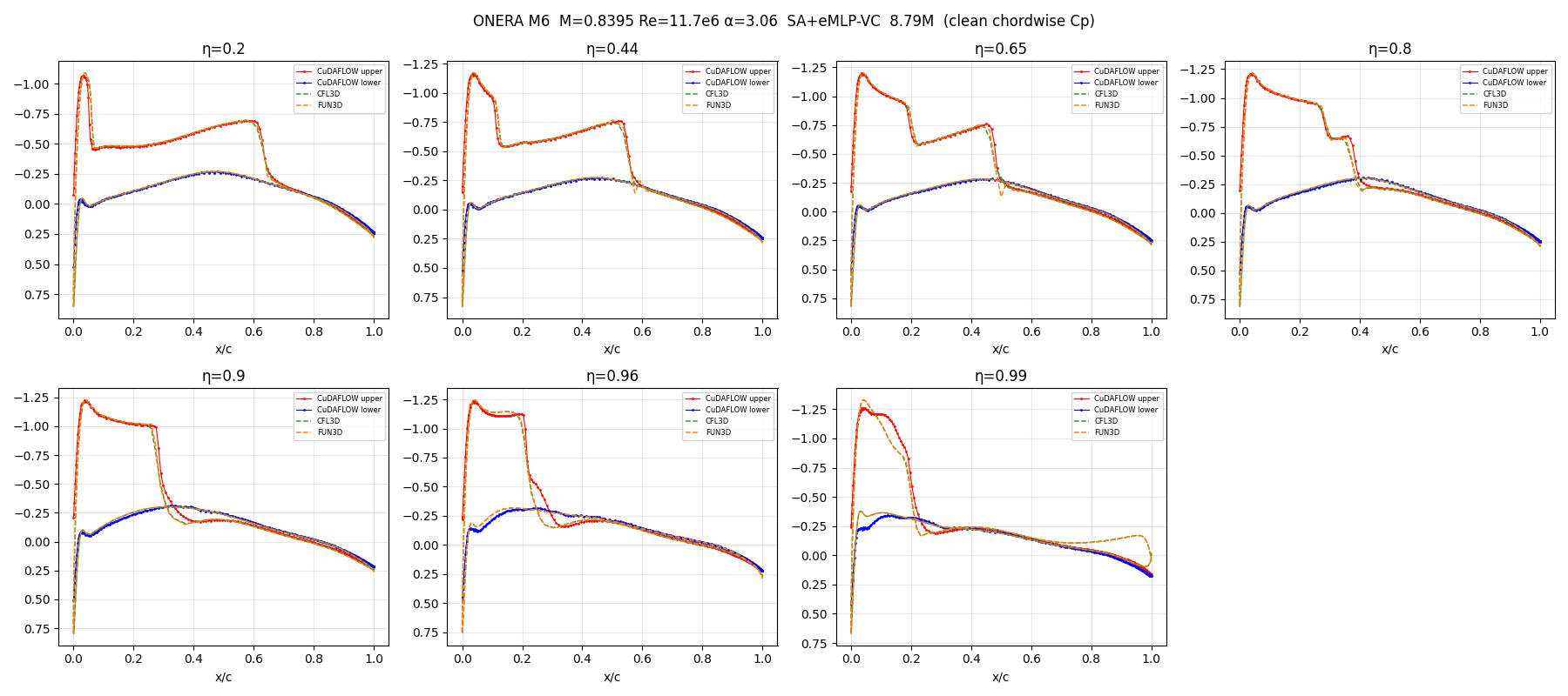
| ONERA M6 transonic wing | M = 0.84, α = 3.06°, multiblock, eMLP-VC | λ-shock captured; surface pressure in line with experiment |
| Exact-AD shape adjoint (NACA 0012) | order 3, viscous, CuAD AD Jacobian + PETSc | Assembly consistency ‖gJac·q − dR‖ ≈ 3.6e-4; shape gradient right-sign, usable |
🔧 Engineering Notes
The core finding is that for the stiff RANS discrete adjoint exact AD is not a luxury: an ill-conditioned adjoint amplifies a 6.85%-accurate finite-difference Jacobian into a 233× gradient error with the wrong sign. CuAD makes every residual derivative exact, and because the amplified terms (∂R/∂Q, ∂R/∂X, ∂R/∂wd) are objective-independent, the same machinery serves shape optimization, Cf/Cp inverse design and Spalart–Allmaras field inversion (FIML) alike — the choice of objective only enters through the (un-amplified) ∂J/∂Q. A regression harness checks the AD-Jacobian assembly consistency, the adjoint convergence, and that the FIML loss actually descends.
GPL-3.0.